라임오렌지파이와 일상

선정논문

• Quantization and Training of Neural Networks for Efficient Integer-Arithmetic-Only Inference, 2017
• Integer Quantization for Deep Learning Inference: Principles and Empirical Evaluation, 2020

Integer Quantization for Deep Learning Inference: Principles and Empirical Evaluation

Part 2.1 – Related Works

• ICLR 2018, Baidu&NVIDIA, Mixed precision training: 기존 FP32 Datatype이 아닌 FP16에서 Training할 수 있도록 하는 Technique
• 2011, Google, Improving the speed of neural networks on CPUs: 최신 x86 CPU Inference를 최적화하기 위해 CPU에 내장된 최신 연산 SSE2, SSSE3, SSE4를 활용하여 4~10배의 성능 향상 및 Fixed-point Instruction이 가능한 Specialized Hardware에서 높은 성능 향상 기대
• 📜CVPR 2018, Quantization and training of neural networks for efficient integer-arithmetic-only inference: 모든 Inference를 INT 연산으로만 진행하여 모델을 최적화하는 기법
• 2018, Quantizing deep convolutional networks for efficient inference: A whitepaper: Inference를 위한 Quantization 기법. Post-Training Quantization(PTQ)과 Quantization Aware Training(QAT)를 MobileNet에 각각 적용하여 실험함함
• 2018, PACT: Parameterized Clipping Activation for Quantized Neural Networks: Training Time에 각 Weight의 Activation range를 학습하여 Quantization에 사용함

Part 2.2 – Known Facts / Miscellaneous

• 처음/마지막 레이어는 Quantization하지 않음 (Quantization에 민감함)
• Quantization에는 Uniform, Non-uniform Quantization이 있음
• LSTM, RNN에서 적용했을 때 PTQ 방식이 더 성과가 있었음
• MobileNetV2에서도 마찬가지로 PTQ 방식에서 성과가 있었음
• KL-Divergence 문제를 해결하여 Quantization range를 결정하는 방식도 있음
• So on… (논문 참조)

Part 3 – Fundementals

균일(Uniform) 양자화를 이용하여 Float-range의 값을 Integer-range의 값으로, 아래 총 두 단계에 걸쳐서 Mapping을 진행합니다.
1단계로 양자화를 할 실수(Float)의 범위(=Activation range)를 지정하고, 이외의 값은 Clamp(최대/최소값 고정)를 수행합니다.
2단계로 실수-정수 매핑을 수행합니다. 양자화를 수행할 때 가장 가까운 실수와 매핑합니다(Mapping real value to the cloest integer value).

• Quantize: 실수→양자회된 정수 표현 (fp32→int8)
• Dequantize: 양자화된 정수→실수 표현 (int8→fp32)

• Range Mapping: f(x)=s*x+z 의 형태로 실수(x)를 정수 공간으로 매핑합니다. 이를 Affine Quantization 방식이라고 하며, z=0인 특수한 경우를 Scale Quantization 방식이라고 합니다.

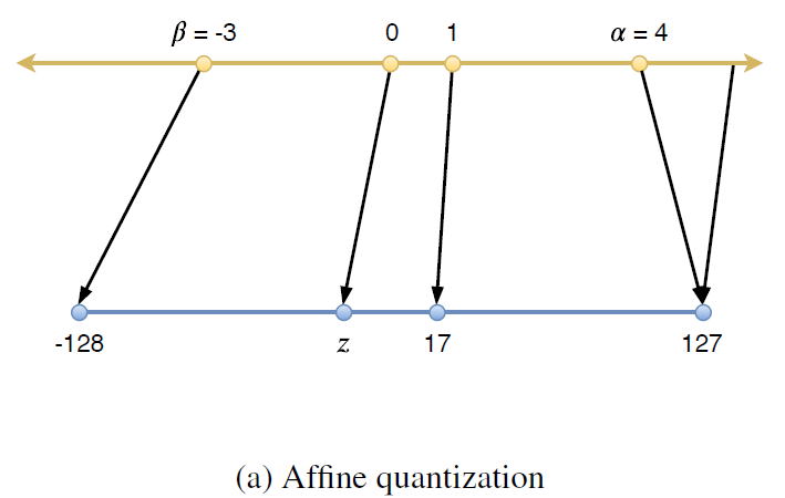
z의 경우 영점(0)을 의미하는데, 어떤 정수 값이 실수 0에 매핑되는지를 결정합니다. 실수의 0에 해당하는 값을 보정하는 역할을 합니다.

전체 Quantization 과정은 (4)와 같습니다. round()는 실수를 가장 가까운 정수로 매핑합니다. 이렇게 양자화된 값을, 반대로 역양자화(Dequantize)하여 해당하는 실수값과의 차이를 계산할 수 있습니다.

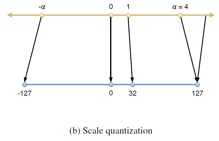
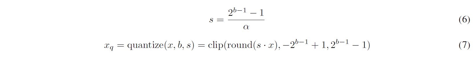
Scale Quantization의 경우 “z”값 없이 scale만을 quantize합니다. 영점이 이동하지 않으므로 z를 구해주거나 더해주는 연산이 줄어들게 됩니다. 보통 Symmetric Quantization이라고도 하는데, 실수공간과 정수공간이 동일하게 0을 중심으로 하게 됩니다. 논문에서는 signed int8 type을 이용하여, Symmetric(대칭크기)을 위해 -128을 제외하고 -127~127까지를 사용합니다.

여기서 Dequantization에 사용되는 수식은 아래와 같습니다.

• Tensor Quantization Granularity: Tensor Quantization에서 parameter (s, z 또는 s)를 어떤 context까지 사용할 것인지를 의미합니다. 예로, Finest granularity는 Element-wise로 parameter를 가질 것이며, Intermediate granularity는 Tensor의 Dimension-wise로 parameter를 가질 것입니다 (같은 Dimension이라면 같은 Parameter를 가짐).
  → Granularity를 결정하는 Factor: Model Accuracy Impact Factor, Computational Cost
  …TBR
• Computational Cost of Affine Quantization

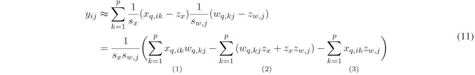
Affine Quantization을 MatMul으로 개념을 확장하여 풀어서 쓰면 (11)과 같습니다. 이 때, MAdd 연산을 총 3개로 분할할 수 있습니다. (1)은 Int8(Activation Map)*Int8(Weight) 연산이며, (2)는 Zero-point multiplication 연산입니다. bias 역시 weight의 일부이므로 여기에 포함됩니다. (1)의 경우 필수적이며, (2)의 경우 각 term이 weight와 zero point로만 이루어져 있으므로 선계산(compute offline)하여 Inference time을 줄일 수 있습니다. 다만 마지막 (3) term의 경우 입력 Activation과 Zero point의 multiplication 연산이므로, Extra cost를 유발합니다.
→ Zero-point를 고려하기에는 Computational Cost가 높아져 버리는 효과를 발생함

따라서, 논문은 되도록이면 Scale quantization을 사용할 것을 권장합니다. 또한 논문의 실험에 따르면 모든 네트워크가 INT8 Quantization task에서는 Scale quantization만으로도 충분하다고 합니다.

• Calibration: 입력값범위(alpha, beta)를 찾는 과정입니다. 이 값은 Activation map(입력 레이어)의 값들의 범위를 한정하는 역할을 합니다. 다만 Scale quantization에서는 이 범위가 Symmetric이므로, 값이 alpha=beta로 한정됩니다. 찾는 방식은 {Max, Entropy, Percentile}이 있습니다.
  (물론 Activation 값들을 나열할 때는 Absolute Value로 나열될 것입니다.)
  • Max: 보여진 값들 중 가장 큰 값
  • Entropy: Quantization을 진행할 때 표현되는 값들의 정보손실이 최소화되는 KL-Divergence를 수행하여, 해당 값을 취합니다. TensorRT에서는 이 방식이 기본적으로 사용된다고 합니다.
  • Percentile: n%의 값들을 취하고, 나머지 (100-n)%에 해당하는 값들은 Clip해버립니다.

Part 4 – Post Training Quantization

…TBR

• Weight Quantizationn
• Activation Quantization

Part 5 – Techniques to Recover Accuracy

…TBR

• Partial Quantization
• Quantization-Aware Training (QAT): …TBR

• Learning Quantization Parameters

Part 6 – Recommended Workflow

TBR…

Part 7 – Conclusion

TBR…